Classifying Biomedical Data Analysis Using Python Code
Section 1: Nearest Neighbor Algorithm
The Nearest Neighbor Algorithm is an effective algorithm for classification. The idea is relatively simple. If we have a data point, we can put the data point on a scatterplot with a specified x and y coordinate. From there, we can use and find neighboring points or the nearest point in the scatterplot to check the classification of it, and predict that our data point should have the same classification as that of the nearest point.
In this project, the Nearest Neighbor Algorithm looked something like this: (1) determine which point in the training data is closest to the new point being tested. This was done by calculating the distance from the new point to the other data set points as well as finding the point that is the minimum distance by looping through all the training data and keeping track of the shortest distance and the point that produced that distance. (2) Then, returning the classification of the nearest point and labeling it respectively to the data set provided.
Some advantages of the Nearest Neighbor Algorithm is that: (1) it’s an extremely effective algorithm. Instead of having to loop through the data hand by hand by yourself, having a computer to use a program and functions to loop through is much easier and saves time. (2) It is also sometimes better to use than the K-Nearest Neighbor Algorithm as sometimes if the data point is right in the middle of a tie between two outcomes, the last KNN tiebreaker odd number value of K may not have been the best way to resolve the category of the data point. BUT the disadvantage that KNN has over the Nearest Neighbor Algorithm is that having more points to compare to does make a difference and can be an effective way of classification.
Section 2: K-Nearest Neighbor Algorithm
The K-Nearest Neighbor Algorithm assumes that similar things exist in close proximity. In other words, similar things are near each other. It captures the idea of similarity (sometimes called distance, proximity, or closeness) with some mathematics we learned in our childhood— calculating the distance between points on a graph.
The K-Nearest Neighbor Algorithm sounds a little bit like this: loading in the data and initializing K to be your chosen number of neighbors. For each example in the data, calculate the distance between the query example and the current example from the data and add the distance and the index of the example to an ordered collection. Additionally, you want to sort the ordered collection of distances and indices from smallest to largest by the distances, pick the first K entries from the sorted collection, get the labels of the selected K entries. In classification, you will return the mode of the K labels.
The main difference between the K-Nearest Neighbor Algorithm and the Nearest Neighbor Algorithm is that we can specify the right value for K (must be an odd number to break ties). As we decrease the value of K to 1, our predictions become less stable. Inversely, as we increase the value of K, our predictions become more stable due to majority averaging.
Some advantages of the K-Nearest Neighbor Algorithm is that: (1) the algorithm is simple and easy to implement, (2) there’s no need to build a model, tune several parameters, or make additional assumptions, and (3) the algorithm is versatile. BUT there are disadvantages: for example, the algorithm gets significantly slower as the number of examples and/or predictors/independent variables increase.
A Side by Side Comparison of When Nearest Neighbor is Better Than K-Nearest Neighbor:
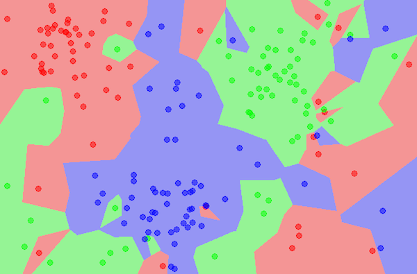
Although K-Nearest Neighbor often gets the impression of being “better” than the Nearest Neighbor Algorithm, here we see an example of when this is not the case. In this example, the k value for K-Nearest Neighbor was set to 7. As you can see, although 7 for K-Nearest Neighbor shows that the patient would be diagnosed for CKD, in the Nearest Neighbor, we see the exact opposite where the closest point to the patient is not CKD (the correct diagnosis). So, both of these algorithms have their fair share of pros and cons.

Figure 1. An Example of When the Nearest Neighbor Algorithm Would Be Better Suited as Method of Classification.
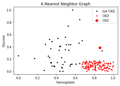
Figure 2. An Example of When K-Nearest Neighbor is Not the Best Choice of Classification.
Section 3: K-Means Clustering Algorithm
Part 1: A Brief Description of my K-Means Clustering Functions
Here is a basic rundown of the K-Means Clustering Functions:
Select: begin by selecting k random centroid points, falling within the range of the feature set
Assign: then, assign to each data point a label based on the centroid is it closest too
Update: take the means of all features of all data points currently assigned to that centroid
Iterate: repeat the assign and update steps until an end condition is met
All of this is described in more detail below in Part 3.
Part 2: The General Algorithm Used
The general algorithm for the K-Means Clustering method is as follows: (1) choose the number of clusters k, (2) select k random points from the data as centroids, (3) assign all the points to the closest cluster centroid (the distance formula is used here), (4) recompute the centroids of newly formed clusters, and lastly (5) repeat steps 3 and 4.
To be specific, here is a rundown of each step in more detail: (1) randomly initialize the centroids of each cluster from the data points (the random function was used here to generate the initial centroids), (2) for each data point, use the distance formula to compute the distance from all the centroids (a for loop and an array were used here to keep track of each step in the append process), (3) adjust the centroid of each cluster by taking the average of all the data points which belong to that cluster on the computations done in step 2 (another for loop was used here to update the centroid positions as well as the mean function), (4) finally, repeat the process until convergence is achieved/an endpoint is reached (a while loop was used until maximum iteration was reached).
An important part to note about the K-Means Clustering Algorithm is that it is different from Nearest Neighbor and K-Nearest Neighbor because there must be a stopping criteria for K-Means Clustering. There are three stopping criteria that can be adopted to stop the K-Means algorithm: (1) centroids of newly formed clusters do not change, (2) points remain in the same cluster, or (3) maximum number of iterations are reached.
There are a lot of benefits to using the K-Means Clustering Algorithm; for example, it has many applications in the real world, from recommending songs on Spotify to finding trends in the stock market and banks. The one disadvantage to using the K-Means Clustering Algorithm is that clusters are drawn and developed through linear lines that divide the groups, meaning that if I had a line that was supposedly squiggly or curved that divided the groups, this algorithm would not be able to form clusters based on that squiggly or curved line. Another disadvantage is that random initialization in step 1 is not an effective way to start with, as sometimes it leads to increased numbers of required clustering iterations to reach convergence, a greater overall runtime, and a less-efficient algorithm overall.
Part 3: Example Graphs

Figure 3. One Cluster K-Means Clustering Graph.

Figure 4. Two Cluster K-Means Clustering Graph.

Figure 5. Three Cluster K-Means Clustering Graph.
Part 4: K-Means Clustering Algorithm Accuracy for the 2 Clusters Condition

Figure 6. K-Means Clustering Accuracy.
My K-Means Clustering Algorithm is pretty accurate, mostly returning close to 100% true positives and true negatives rates. Sensitivity measures the proportion of actual positives that are correctly identified. Specificity measures the proportion of negatives that are correctly identified. In an ideal world, we want both of these percentages to be 100% to ensure 100% accuracy. Comparing these cluster assignments to the human labels from the CSV file, this algorithm is pretty close and impressive in being able to predict a patient’s classification.
Question: Consider if you were designing a medical diagnostic tool --- which of these statistics would be the most important to minimize or maximize in your design?
If I were designing a medical diagnostic tool, I would keep in mind the pros and cons of each algorithm when considering which statistics would be the most important to my design.
Firstly, let’s consider the Nearest Neighbor Algorithm. While this method is extremely useful, there are some flaws to its design. In the real world, you can’t just compare a patient’s data to the nearest point that they are most similar to. That can prove to be extremely harmful and dangerous, as sometimes there are outliers in the data, and not everything can be divided into two clean sections— like in this project example.
Secondly, let’s consider the K-Nearest Neighbor Algorithm. Although this method proves to be effective, as indicated in one of the images above (comparing KNN and NN), there are flaws, especially if the k value is wrong (too small or too large). Yes, looking at your “fellow neighbors” is a good help to understanding where a patient’s data lies, but again, in the real world, unpredictability is more prevalent than not.
Lastly, let’s consider the K-Means Clustering Algorithm. Although this method is a neat way to classify groups into subgroups through the use of centroids, there are flaws, especially because the data is divided by a linear line when there could be in fact a better line (squiggly or curved) that can classify the data into subgroups.
If I could design a medical diagnostic tool, I would take the pros of these three methods and maximize them by combining them into one. The pros: (1) effectiveness of a computer program and (2) ability to rely on neighbors to make a realistic estimate. However, I would minimize the cons as much as possible by finding a way to have K-Means Clustering use more than one type of linear line (perhaps an infinitesimal number of lines to make a curve to divide/classify specific groups). The key to medical diagnostic tools is that they must be realistic as they are applicable to the real world and situations of life and death diagnosis.